Simplifying Differentiation using Directed Acyclic Graphs

Differentiation is easy, right? I always thought so. But then came complex derivatives in the form of Backpropagation and Backpropagation through Time. If you also think differentiation is easy, I urge you to try out deriving Backpropagation through Time before reading ahead.

In this blog, I shall walk you through modelling mathematical functions as Directed Acyclic Graphs, and then finding their derivatives. This is something I learned as part of the course Computational Differentiation at RWTH Aachen University, taught by Prof. Uwe Naumann. This method made it extremely easy to derive Backpropagation algorithms in Deep Learning.

Let us start by recalling the chain rule of differentiation once.

$$y = \mathbf{f}(\mathbf{g}(x))$$ $$\frac{dy}{dx} = \frac{d\mathbf{f}(\mathbf{g})}{d\mathbf{g}} \cdot \frac{d\mathbf{g}(x)}{dx}$$

Now, try deriving the following:

$$y = x \cdot e^{sin(x)}$$

How do Directed Acyclic Graphs come into the picture?

A Directed Acyclic Graph can be used to graphically represent the computation of a mathematical function. Each node of the graph represents an elementary computation. Edges represent the flow of computations.

We shall start by reducing the function given above into elementary computations known as Single Assignment Code.

Single Assignment Code

A SAC of a mathematical function is a multi-step computation, where in each step, only one elementary computation may be performed. A single application of +, -, *, /, log, exp, sin, cos etc. may be termed as an elementary computation.

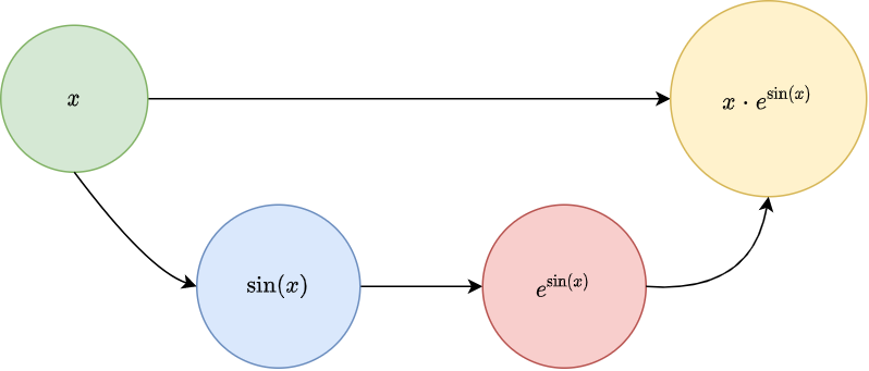
For example, $$y = x \cdot e^{sin(x)}$$

The Single Assignment Code for this function: $$v_1 = sin(x)$$ $$v_2 = e^{v_1}$$ $$y = x \cdot v_2$$

Drawing a DAG is pretty simple once we have the SAC for the function. Each assignment in the SAC is a node in the DAG. The edges shall be directed from the inputs to the outputs for each assignment.

As one can notice from the graph, the whole computation is embedded in the graph itself. This means we can compute the result of the function for a certain value of input from the DAG without actually looking at the mathematical form of the function. This DAG is also know as the Computational Graph of the given function.

Enter Derivatives!

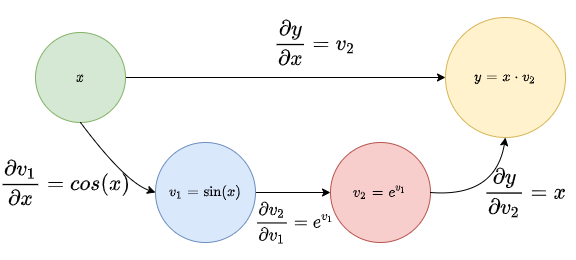
Since we have the computational graph of the function, we just need a slight tweak to the graph to help us get the derivative. Label each edge with the partial derivative of the output node for that edge with respect to the input node for the edge. Notice the word PARTIAL. Since each node is an elementary computation, there is no chain rule involved in computing this derivative.

Derivative of the function from the Computational Graph

Assume we have two nodes i and j in the graph, and there exists a path from i to j. To compute the derivative of j with respect to i, do the following:

1. Traverse each path k from node i to node j in the computational graph and compute the product of the value on each edge on the path. Call it p_k.
2. Compute the sum of the values of p_k for all such paths from i to j.

For our example, we need to compute the derivative of y with respect to x. Traversing the path on the top in the graph, $$p_1 = \frac{\partial y}{\partial x} = v_2$$

Traversing the path at the lower end, $$p_2 = \frac{\partial v_1}{\partial x} \cdot \frac{\partial v_2}{\partial v_1} \cdot \frac{\partial y}{\partial v_2} = cos(x) \cdot e^{v_1} \cdot x$$

So, the required derivative becomes $$\frac{\partial y}{\partial x} = p_1 + p_2$$ $$\frac{\partial y}{\partial x} = (v_2) + (cos(x) \cdot e^{v_1} \cdot x)$$ $$\frac{\partial y}{\partial x} = (v_2) + (cos(x) \cdot e^{v_1} \cdot x)$$ Substituting the values from the SAC, $$\frac{\partial y}{\partial x} = (e^{v_1}) + (cos(x) \cdot e^{sin(x)} \cdot x)$$ $$\frac{\partial y}{\partial x} = (e^{sin(x)}) + (cos(x) \cdot e^{sin(x)} \cdot x)$$.

Simple right? Isn’t it the same thing you get when applying chain rule directly? In fact, whatever we did in the form of Single Assignment Code, Computational Graph and then summing the product of each path was basically the chain rule. I’d leave it to you to think why this actually works. I’d be happy to discuss this personally.

Answer this. What would happen if there is no path from input to output?

Conclusion

We saw how to model computations in the form of computational graphs and compute derivative of any differentiable function. Now, you must be thinking why go through all this when you could directly apply Chain-rule and get the answer? The simple answer is do what is easier. For simple functions, directly applying chain-rule is easier. For, more complex, multi-dimensional functions, Computational Graphs make life super-simple. With a little practice, you can directly jump to drawing the DAG without explicitly using the Single Assignment Code.

Take some complicated functions and try finding the derivatives using the computational graph.

Finally, there are some problems where you are directly given the Computational Graph and you need to find the derivative. The best examples are Multi-layer Perceptrons and Recurrent Neural Networks. It is quite tedious to derive the backpropagation algorithms for these. Now, using the computational graph (in this case, the architecture diagram itself), we can easily derive the backpropagation algorithm. I urge you to try it out. I’ll discuss these in a later tutorial.

Thank you for reading. Please let me know what you think about the post. :)